Quick Start

To get started with pymgrid, first clone or install the package.

This notebook shows how to define a simple microgrid, create actions to control it, and read the results. Microgrids can be defined by either defining a set of modules and then passing them to the Microgrid constructor or by a YAML config file. We detail the first case here.

import numpy as np
import pandas as pd

np.random.seed(0)

from pymgrid import Microgrid
from pymgrid.modules import (
    BatteryModule,
    LoadModule,
    RenewableModule,
    GridModule)

Defining a Microgrid

We can then define some components of our microgrid. We will define two batteries, one with a capacity of 100 kWh and another with a slower charging rate and lower efficiency but a capacity of 1000 kWh.

small_battery = BatteryModule(min_capacity=10,
                              max_capacity=100,
                              max_charge=50,
                              max_discharge=50,
                              efficiency=0.9,
                              init_soc=0.2)

large_battery = BatteryModule(min_capacity=10,
                              max_capacity=1000,
                              max_charge=10,
                              max_discharge=10,
                              efficiency=0.7,
                              init_soc=0.2)

We will also define a load and photovoltaic (pv) module – the latter representing, say, a solar farm – with some random data. We will define 90 days worth of data, in hourly increments.

load_ts = 100+100*np.random.rand(24*90) # random load data in the range [100, 200].
pv_ts = 200*np.random.rand(24*90) # random pv data in the range [0, 200].

load = LoadModule(time_series=load_ts)

pv = RenewableModule(time_series=pv_ts)

Finally, we define an external electrical grid to fill any energy gaps.

The grid time series must contain three or four columns. The first three denote import price, export price, and carbon dioxide production per kWh. If a fourth column exists, it denotes the grid status (as a bool); if it does not, the grid is assumed to always be up and running.

grid_ts = [0.2, 0.1, 0.5] * np.ones((24*90, 3))

grid = GridModule(max_import=100,
                  max_export=100,
                  time_series=grid_ts)

We can then pass these to the Microgrid constructor to define a microgrid. Here, we give our renewable module the name “pv”.

modules = [
    small_battery,
    large_battery,
    ('pv', pv),
    load,
    grid]

microgrid = Microgrid(modules)

Printing the microgrid will tell us the modules contained in that microgrid. By default a balancing module is added to keep track of any unmet demand or excess production. This can be disabled by passing unbalanced_energy_module=False, but is not recommended.

print(microgrid)

Microgrid([load x 1, pv x 1, balancing x 1, battery x 2, grid x 1])

We can then access the modules in the microgrid by name or by key:

print(microgrid.modules.pv)

[RenewableModule(time_series=<class 'numpy.ndarray'>, raise_errors=False, forecaster=NoForecaster, forecast_horizon=0, forecaster_increase_uncertainty=False, provided_energy_name=renewable_used)]

print(microgrid.modules.grid is microgrid.modules['grid'])

True

Controlling a microgrid

You must pass an action for each controllable module to control the microgrid. The fixed modules are stored in the attribute microgrid.controllable:

microgrid.controllable

{
  "battery": "[BatteryModule(min_capacity=10, max_capacity=100, max_charge=50, max_discharge=50, efficiency=0.9, battery_cost_cycle=0.0, battery_transition_model=None, init_charge=None, init_soc=0.2, raise_errors=False), BatteryModule(min_capacity=10, max_capacity=1000, max_charge=10, max_discharge=10, efficiency=0.7, battery_cost_cycle=0.0, battery_transition_model=None, init_charge=None, init_soc=0.2, raise_errors=False)]",
  "grid": "[GridModule(max_import=100, max_export=100)]"
}

As we can see, our “load”, “battery”, and “grid” modules are fixed.

We can also view what modules we need to pass an action for by getting an empty action from the microgrid. Here, all None values must be replaced to pass this action as a control.

print(microgrid.get_empty_action())

{'battery': [None, None], 'grid': [None]}

We can then simply define a control for these modules. Before doing so, we will reset our microgrid and then check its current state.

microgrid.reset()
microgrid.state_series.to_frame()

			0
load	0	load_current	-169.646919
pv	0	renewable_current	65.358668
battery	0	soc	0.200000
		current_charge	20.000000
	1	soc	0.200000
		current_charge	200.000000
grid	0	import_price_current	0.200000
		export_price_current	0.100000
		co2_per_kwh_current	0.500000
		grid_status_current	1.000000

We will attempt to meet our load demand of 169.646919 by using our available renewable and then discharging our batteries:

load = -1.0 * microgrid.modules.load.item().current_load
pv = microgrid.modules.pv.item().current_renewable

net_load = load + pv # negative if load demand exceeds pv

if net_load > 0:
    net_load = 0.0

For our batteries, we will attempt to generate the lower of the excess load and the maximum production.

battery_0_discharge = min(-1*net_load, microgrid.modules.battery[0].max_production)
net_load += battery_0_discharge

battery_1_discharge = min(-1*net_load, microgrid.modules.battery[1].max_production)
net_load += battery_1_discharge

Finally, we will let our grid clean up the rest – or as must as it can.

grid_import = min(-1*net_load, microgrid.modules.grid.item().max_production)

Putting this together, we have our control.

Note that positive values denote energy moving into the microgrid and negative values denote energy leaving the microgrid.

control = {"battery" : [battery_0_discharge, battery_1_discharge],
           "grid": [grid_import]}

control

{'battery': [9.0, 7.0], 'grid': [88.28825060785877]}

We can then run the microgrid with this control. Since this control is not normalized, we pass normalized=False.

obs, reward, done, info = microgrid.run(control, normalized=False)

Analyzing Results

After passing a control to the microgrid, we can view the results by viewing the microgrid’s – or any of the modules – logs.

The microgrid’s log has one row for each action taken. There are values for both the actions – e.g. the amount of load met – as well as the state: for example, the current load.

Note that the state values are the values of the state from before the action was taken.

The columns are a pd.MultiIndex, with three levels: module names, module name enumeration (e.g. which number of each module name we are in) and property.

For example, since there is one load, all of its log entries will be available under the key ('load', 0). Since there are two batteries, there will be both (battery, 0) and (battery, 1).

We can see that we met all of our load:

microgrid.log.loc[:, pd.IndexSlice['load', 0, :]]

module_name	load
module_number	0
field	reward	load_met	load_current
0	0.0	169.646919	-169.646919

And consumed all available pv, even though we did not define a control for it:

microgrid.log.loc[:, pd.IndexSlice['pv', 0, :]]

module_name	pv
module_number	0
field	reward	curtailment	renewable_used	renewable_current
0	0.0	0.0	65.358668	65.358668

Since we have two batteries, we will have log entries for each of them:

microgrid.log.loc[:, 'battery']

module_number	0					1
field	reward	discharge_amount	charge_amount	soc	current_charge	reward	discharge_amount	charge_amount	soc	current_charge
0	-0.0	9.0	0.0	0.2	20.0	-0.0	7.0	0.0	0.2	200.0

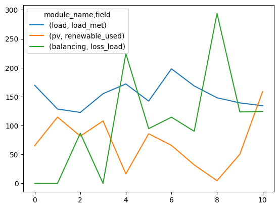
Plotting Results

We can also utilize pandas plotting functionality to view results. To illustrate this, we will run the microgrid for an additional ten steps with randomly sampled actions.

for _ in range(10):
    microgrid.run(microgrid.sample_action(strict_bound=True))

Here we will plot the load met, pv consumed and loss load:

microgrid.log[[('load', 0, 'load_met'),
               ('pv', 0, 'renewable_used'),
               ('balancing', 0, 'loss_load')]].droplevel(axis=1, level=1).plot()

<AxesSubplot:>